NLP_Visualization and Classification.

Natural Language Processing (NLP), gives computers the ability to understand text and spoken words in much the same way human beings can. It combines computational linguistics—rule-based modeling of human language with statistical, machine learning, and deep learning models.

Loading all the necessary packages

import matplotlib.pyplot as plt
%matplotlib inline
import numpy as np
import pandas as pd
import spacy
import seaborn as sns
import plotly.offline as py
color = sns.color_palette()
import plotly.graph_objs as go
py.init_notebook_mode(connected=True)
import plotly.tools as tls

Reading in the Data

# Load the large model to get the vectors
nlp = spacy.load('en_core_web_lg')

review_data = pd.read_csv('../input/nlp-course/yelp_ratings.csv')

Viewing the first five rows of the data using “.head()”

review_data.head()

index	text	stars	sentiment
0	Total bill for this horrible service? Over $8G…	1.0	0
1	I adore Travis at the Hard Rock’s new Kelly …	5.0	1
2	I have to say that this office really has it t…	5.0	1
3	Went in for a lunch. Steak sandwich was delici…	5.0	1
4	Today was my second out of three sessions I ha…	1.0	0

Visualization

Word Cloud

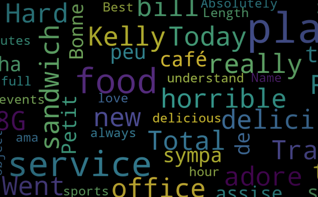
These shows a representation of the text data as an image made of words. Words that are more important or rather more frequent are usually larger. It gives us a basic overview of the text data in a visually appealing manner.

from wordcloud import WordCloud, STOPWORDS
stopwords = set(STOPWORDS)

def show_wordcloud(data, title = None):
    wordcloud = WordCloud(
        background_color='black',
        stopwords=stopwords,
        max_words=200,
        max_font_size=40, 
        scale=3,
        random_state=1 
).generate(str(data))

    fig = plt.figure(1, figsize=(15, 15))
    plt.axis('off')
    if title: 
        fig.suptitle(title, fontsize=20)
        fig.subplots_adjust(top=2.3)

    plt.imshow(wordcloud)
    plt.show()

show_wordcloud(review_data['text'])

word cloud

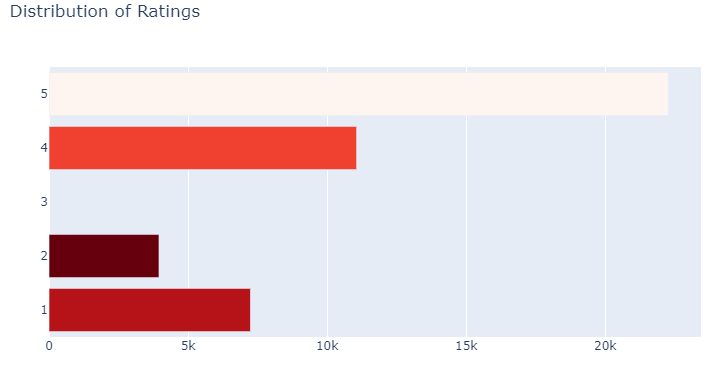
It would also be interesting to see the distribution of the ratings. The ratings for three stars have been droppped since they cannot be of much help as they are neutral. They don’t give a strong standpoint with their reviews.

py.init_notebook_mode(connected=True)

cnt_srs = review_data['stars'].value_counts().head()
trace = go.Bar(
    y=cnt_srs.index[::-1],
    x=cnt_srs.values[::-1],
    orientation = 'h',
    marker=dict(
        color=cnt_srs.values[::-1],
        colorscale = 'reds',
        reversescale = True
    ),
)

layout = dict(
    title='Distribution of Ratings',
    )
data = [trace]
fig = go.Figure(data=data, layout=layout)
py.iplot(fig, filename="Ratings")

distrib of ratings

Hmmm, apparently there are alot of positive sentiments ,i.e the 5-star and 4-star are quite many. Its quite apparent that the servings are of acceptable quality.

Heatmap

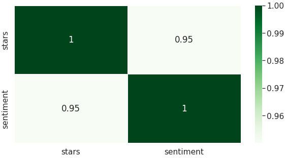
We can also view the correlation between the variables.

sns.set(font_scale=1.4)
plt.figure(figsize = (10,5))
sns.heatmap(review_data.corr(), cmap='Greens',annot=True,linewidths=.5)

correlation

document vectors

We will use the first 100 document vectors.

reviews = review_data[:100]
# We just want the vectors so we can turn off other models in the pipeline
with nlp.disable_pipes():
    vectors = np.array([nlp(review.text).vector for idx, review in reviews.iterrows()])
    
vectors.shape

(100, 300)

The resultant matrix is a (100 by 300)

We can now load all the document vectors so that we can begin training our model.

vectors = np.load('../input/nlp-course/review_vectors.npy')

Training Model

On document Vectors

We are going to use a supervised classification method known as Support Vector Machine…specifically Linear Support Vector Classification. They are usually quite effective on high dimensional spaces.

from sklearn.svm import LinearSVC
from sklearn.model_selection import train_test_split

X_train, X_test, y_train, y_test = train_test_split(vectors, review_data.sentiment, 
                                                    test_size=0.1, random_state=1)

# Creating the LinearSVC model
model = LinearSVC(random_state=1, dual=False)
# Fitting the model
model.fit(X_train, y_train)

LinearSVC(dual=False, random_state=1)

Now we can now test its accuracy with the ‘hold-out’ data.

Model Accuracy in Test Data

# model accuracy on test data
print(f'Model test accuracy: {model.score(X_test, y_test)*100:.3f}%')

Model test accuracy: 93.847%

The model does seem to classify the data in a highly accurate manner.