Time Series Analysis.

“Predicting the future is easy… It’s trying to figure out what’s going on now that’s hard!”

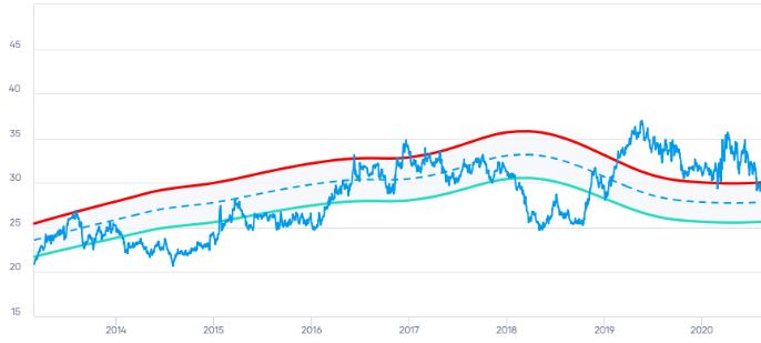
Data that is gathered over time at regular intervals are analyzed using the statistical technique known as time series analysis. It entails examining patterns and trends in the data to comprehend the underlying causes of those patterns. Time series analysis is frequently utilized in many disciplines, including signal processing, finance, economics, and weather forecasting.

It can be used to predict

Sales and revenue based on past trends and seasonality.
Stock prices based on historical trends and market conditions.
Economic indicators such as GDP, inflation, and unemployment rates.
Weather patterns based on past climate data.
Traffic patterns on highways and other transportation systems based on historical data.
Demand for products and services based on past trends and seasonality.
Energy consumption based on historical data and weather patterns.
Web traffic to a website based on historical data and seasonality patterns.
Resource utilization such as server usage, network bandwidth, and storage capacity based on past trends.
Customer churn rates based on historical data and customer behavior patterns.
Marketing campaigns impact on sales based on historical data and campaign performance.
Patient health outcomes based on past medical records and patient data.
Manufacturing output based on past production data and demand trends

Time Series Patterns

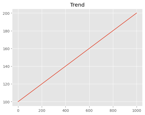
Trend, trend is a long-term increase or decrease in the data over time. It can be linear or nonlinear.

trend

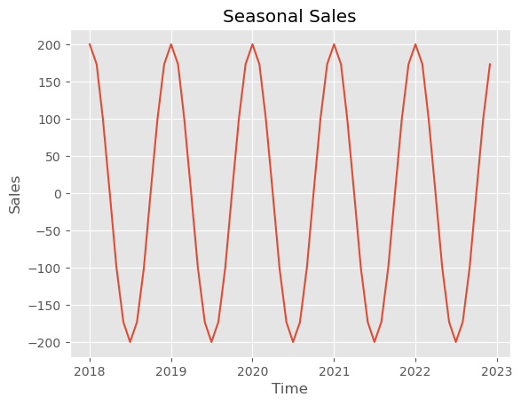
Seasonality, seasonality refers to a pattern that repeats over a fixed time interval, such as daily, weekly, monthly, or yearly.

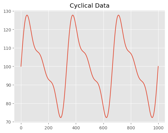
Cyclicality, cyclical patterns are similar to seasonality, but they occur over a longer time frame and may not have a fixed interval. For example, business cycles that last several years can exhibit cyclical patterns.

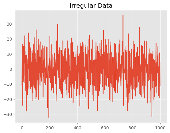
Irregularity, irregular patterns are random fluctuations that cannot be explained by a trend, seasonality, or cyclical pattern. They can be caused by unpredictable events, measurement errors, or other factors.

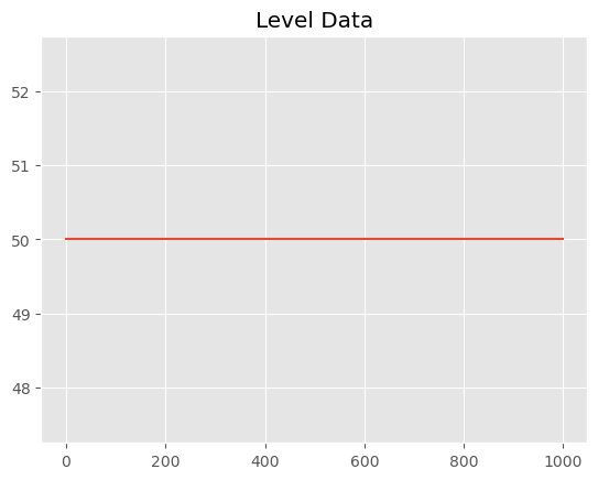
Level, the level of a time series refers to the average value of the series over time. A level pattern can occur when the series has a constant average value.

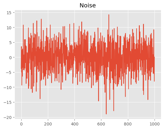
Noise, noise refers to random fluctuations in the data that do not have any underlying pattern. It can be caused by measurement errors, sampling variability, or other sources of random variation.

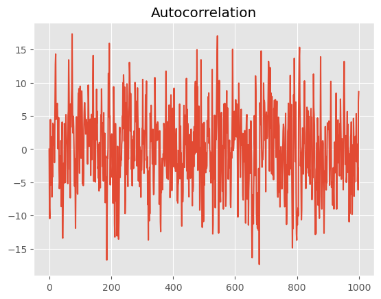
Autocorrelation, this occurs when the values of a time series are correlated with their past values. Autocorrelation can indicate a trend or a cyclical pattern in the data.

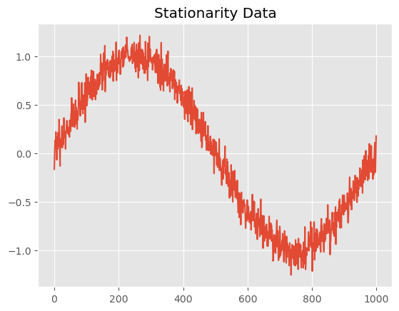
Stationarity, a time series is said to be stationary if its statistical properties, such as its mean and variance, do not change over time. Stationarity is an important property for many time series models, as non-stationary data can be difficult to model and forecast.

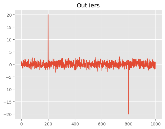
Outliers, these are extreme values in the data that are significantly different from the other values. Outliers can be caused by measurement errors, data entry errors, or other factors. They can affect the accuracy of forecasts and should be identified and removed or corrected if possible.

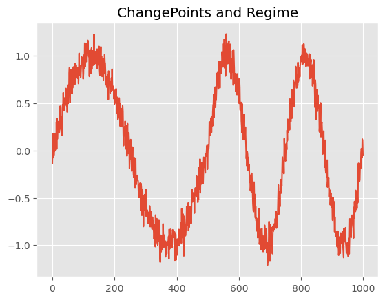
Change points, these are points in time where the pattern of the time series changes abruptly. Change points can be caused by changes in underlying processes or external factors, and they can make it difficult to model and forecast the data.
Regime shifts, they occur when the statistical properties of a time series change over time, such as its mean or variance. Regime shifts can be caused by changes in underlying processes, external factors, or shifts in the way the data is collected or reported.

NB

Change point and regime shift are similar in the sense that they both represent a significant shift or change in the underlying pattern of a time series. However, the difference between the two lies in the duration and nature of the change.A change point is a sudden change or shift in the mean or variance of a time series, which can occur due to a variety of reasons such as an external shock or a change in the underlying process. Change points are typically short-lived and do not have a lasting impact on the overall pattern of the time series. wheareas, a regime shift represents a more fundamental change in the underlying process that generates the time series. Regime shifts are typically longer-lived and can have a lasting impact on the pattern of the time series. Examples of regime shifts include changes in economic policies, technological innovations, or demographic shifts.

Main models in time series analysis

Autoregression (AR), This method uses the past values of a time series to predict future values. The order of the autoregression, denoted by p, specifies the number of past values to use. The AR(p) model can be expressed as a linear combination of past values and a random error term.
Moving Average (MA), This method uses the past errors of a time series to predict future values. The order of the moving average, denoted by q, specifies the number of past errors to use. The MA(q) model can be expressed as a linear combination of past errors and a random error term.
Autoregressive Integrated Moving Average (ARIMA), This method combines the AR and MA models with a differencing step to account for non-stationarity in the time series. The ARIMA(p,d,q) model specifies the order of the autoregression, differencing, and moving average components.
Seasonal Autoregressive Integrated Moving Average (SARIMA), This method extends the ARIMA model to account for seasonality in the time series. The SARIMA(p,d,q)(P,D,Q)s model specifies the order of the seasonal autoregression, seasonal differencing, seasonal moving average, and the length of the seasonal cycle.
Exponential Smoothing (ES), This method uses a weighted average of past values to predict future values. There are several variants of the ES method, including Simple Exponential Smoothing, Holt’s Linear Exponential Smoothing, and Holt-Winters’ Exponential Smoothing. These models differ in their treatment of trend and seasonality.
Prophet, This method is a forecasting procedure implemented in Python and R. It is based on an additive model where non-linear trends are fit with yearly, weekly, and daily seasonality, plus holiday effects. It works best with time series that have strong seasonal effects and several seasons of historical data.
Seasonal Autoregressive Integrated Moving Average with Exogenous Variables (SARIMAX), This method extends the SARIMA model to include exogenous variables, which are external factors that can influence the time series. The SARIMAX(p,d,q)(P,D,Q)s model includes the order of the seasonal autoregression, seasonal differencing, seasonal moving average, the length of the seasonal cycle, and the exogenous variables.
Dynamic Linear Models (DLM), This method is a Bayesian approach to time series prediction that can incorporate prior knowledge about the time series and the forecasting problem. The DLM models the time series as a linear combination of past values, with a state-space model to account for uncertainty in the model parameters.
Gaussian Processes (GP), This method is a non-parametric approach to time series prediction that can model complex nonlinear relationships. The GP model assumes that the time series values are drawn from a Gaussian distribution, with a covariance function that captures the dependencies between past and future values.
Neural Prophet, This method is an extension of the Prophet forecasting procedure that incorporates neural networks for improved accuracy. The Neural Prophet model can be trained using historical data, exogenous variables, and feature engineering techniques.
DeepAR, This method is a deep learning approach to time series prediction that uses a recurrent neural network with an encoder-decoder architecture. The DeepAR model can capture complex dependencies between past and future values, and can incorporate exogenous variables and time-varying covariates.
AutoML, This method is an automated machine learning approach that can automatically select and tune multiple time series prediction models. The AutoML approach can search a large space of model architectures and hyperparameters to find the best-performing model for a given time series.
Prophet AI, This method is a cloud-based time series forecasting platform that uses machine learning and AI algorithms to forecast future trends, patterns and insights in time series data. It can handle large amounts of data and provides both automated and customizable forecasting options.
Long Short-Term Memory (LSTM), This method is a type of recurrent neural network that is well-suited for time series prediction, especially for long-term dependencies. LSTM models have the ability to remember past inputs and selectively forget irrelevant information, making them effective at capturing complex patterns in time series data.
Convolutional Neural Networks (CNN), This method is another type of neural network that is commonly used for image recognition, but can also be applied to time series prediction. The CNN model applies a set of filters to the time series data, which can identify patterns at different scales and levels of abstraction.
Vector Autoregression (VAR), This method is a multivariate time series forecasting technique that models the relationship between multiple time series variables. The VAR model assumes that each variable is a linear function of its own past values and the past values of all other variables in the system.
Bayesian Structural Time Series (BSTS), This method is a Bayesian approach to time series prediction that allows for the inclusion of multiple sources of uncertainty. The BSTS model uses a structural time series approach, which decomposes the time series into trend, seasonal, and irregular components.
Ensemble Methods, This method involves combining multiple time series prediction models to improve overall accuracy. Ensemble methods can be used to combine different types of models, such as ARIMA, LSTM, and CNN, or to combine different versions of the same model with different hyperparameters.
Time Series Clustering, This method involves grouping similar time series together and using a single model to predict the future values of each cluster. Time series clustering can be useful for reducing the computational complexity of the forecasting problem and for identifying patterns and relationships between different time series.
Hybrid Models, This method involves combining multiple forecasting techniques, such as statistical models and machine learning models, to improve the accuracy of time series predictions. Hybrid models can take advantage of the strengths of different models and overcome the weaknesses of individual models.