Titanic Machine learning problem in PYTHON.
April 15, 1912
The widely considered “unsinkable” RMS Titanic met a worthy opponent “iceberg” on her maiden voyage. Due to damages sustained she took a deep dive. Unfortunately, there weren’t enough lifeboats for everyone onboard, resulting in the death of 1502 out of 2224 passengers and crew.
While there was some element of luck involved in surviving, it seems some groups of people were more likely to survive than others.
In this challenge, it is of interest to build a predictive model that answers the question: “what sorts of people were more likely to survive?” using passenger data (ie name, age, gender, socio-economic class, etc).
Loading relevant libraries
import numpy as np # linear algebra
import pandas as pd # data processing, CSV file Input/Output (e.g. pd.read_csv)
from sklearn.impute import SimpleImputer
from sklearn.model_selection import train_test_split
import matplotlib.pyplot as plt
import seaborn as sns
sns.set(style="whitegrid")
import os
for dirname, _, filenames in os.walk('/kaggle/input'):
    for filename in filenames:
        print(os.path.join(dirname, filename))
Loading the training data
train_data = pd.read_csv("/kaggle/input/titanic/train.csv")
train_data.head()
The data.head() line returns a few rows of the whole dataset
Training data
| index | PassengerId | Survived | Pclass | Name | Sex | Age | SibSp | Parch | Ticket | Fare | Cabin | Embarked |
|---|---|---|---|---|---|---|---|---|---|---|---|---|
| 0 | 1 | 0 | 3 | Braund, Mr. Owen Harris | male | 22.0 | 1 | 0 | A/5 21171 | 7.2500 | NaN | S |
| 1 | 2 | 1 | 1 | Cumings, Mrs. John Bradley (Florence Briggs Th… | female | 38.0 | 1 | 0 | PC 17599 | 71.2833 | C85 | C |
| 2 | 3 | 1 | 3 | Heikkinen, Miss. Laina | female | 26.0 | 0 | 0 | STON/O2. 3101282 | 7.9250 | NaN | S |
| 3 | 4 | 1 | 1 | Futrelle, Mrs. Jacques Heath (Lily May Peel) | female | 35.0 | 1 | 0 | 113803 | 53.1000 | C123 | S |
| 4 | 5 | 0 | 3 | Allen, Mr. William Henry | male | 35.0 | 0 | 0 | 373450 | 8.0500 | NaN | S |
Looking at the output for the training data we see that there is alot of Nans in the Cabin column. The rest of the data for the small sample on display looks natural. We will perform more exploratory analysis on them to select features.
Loading the test Data
test_data = pd.read_csv("/kaggle/input/titanic/test.csv")
test_data.head()
Test data
| index | PassengerId | Pclass | Name | Sex | Age | SibSp | Parch | Ticket | Fare | Cabin | Embarked |
|---|---|---|---|---|---|---|---|---|---|---|---|
| 0 | 892 | 3 | Kelly, Mr. James | male | 34.5 | 0 | 0 | 330911 | 7.8292 | NaN | Q |
| 1 | 893 | 3 | Wilkes, Mrs. James (Ellen Needs) | female | 47.0 | 1 | 0 | 363272 | 7.0000 | NaN | S |
| 2 | 894 | 2 | Myles, Mr. Thomas Francis | male | 62.0 | 0 | 0 | 240276 | 9.6875 | NaN | Q |
| 3 | 895 | 3 | Wirz, Mr. Albert | male | 27.0 | 0 | 0 | 315154 | 8.6625 | NaN | S |
| 4 | 896 | 3 | Hirvonen, Mrs. Alexander (Helga E Lindqvist) | female | 22.0 | 1 | 1 | 3101298 | 12.2875 | NaN | S |
Just like for the training data, the test data has many Nans…the rest of the variables look natural.
Some Exploratory analysis.
It is of interest to see the relation with the responce variable “Survived”. This will help us see those variables that affect survival rate which will in turn aid in the modelling. Also it is important as we are able to assess if there is some data leakage inorder to avoid false high accuracy rates and data contamination in overall.
Sex
women = train_data.loc[train_data.Sex == 'female']["Survived"]
rate_women = sum(women)/len(women)

print("% of women who survived:", rate_women)
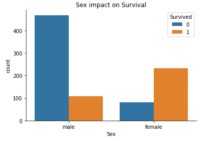
% of women who survived: 0.7420382165605095
men = train_data.loc[train_data.Sex == 'male']["Survived"]
rate_men = sum(men)/len(men)

print("% of men who survived:", rate_men)
% of men who survived: 0.18890814558058924
Sex seems like it has a significant impact on the Survival rate. We can plot the relation.
sns.countplot(x ='Sex', hue = "Survived", data = train_data).set_title("Sex meaning in Survival")
sns.despine()
# SibSp
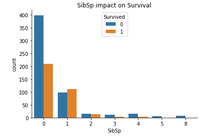
sns.countplot(x ='SibSp', hue = "Survived", data = train_data).set_title("SibSp impact on Survival")
sns.despine()
# # Parch
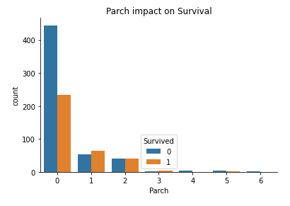
sns.countplot(x ='Parch', hue = "Survived", data = train_data).set_title("Parch impact on Survival")
sns.despine()
# Pclass
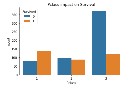
sns.countplot(x ='Pclass', hue = "Survived", data = train_data).set_title("Pclass impact on Survival")
sns.despine()
# Embarked
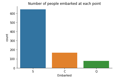
sns.countplot(x ='Embarked', data = train_data).set_title("Number of people embarked at each point")
sns.despine()
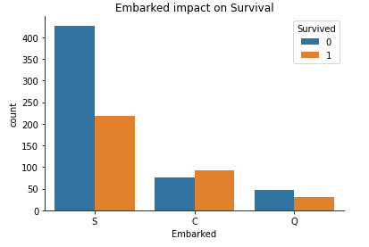
We would like to see the number of people that boarded at each point and how many got to see the light of day with respect to the point of embarking.
train_data["Embarked"] = train_data["Embarked"].fillna("S")

sns.countplot(x ='Embarked', hue = "Survived", data = train_data).set_title("Embarked impact on Survival")
sns.despine()
### Title
# get title for each passenger
train_data["Title"] = train_data.Name.str.extract(' ([A-Za-z]+)\.', expand=False)
test_data["Title"] = test_data.Name.str.extract(' ([A-Za-z]+)\.', expand=False)
# replace synonyms in train_data
train_data['Title'] = train_data['Title'].replace('Mlle', 'Miss')
train_data['Title'] = train_data['Title'].replace('Ms', 'Miss')
train_data['Title'] = train_data['Title'].replace('Mme', 'Mrs')

# replace synonyms in test_data
test_data['Title'] = test_data['Title'].replace('Mlle', 'Miss')
test_data['Title'] = test_data['Title'].replace('Ms', 'Miss')
test_data['Title'] = test_data['Title'].replace('Mme', 'Mrs')

#apply title to dataframe title column
titles = ["Mr", "Mrs", "Miss", "Master"]
train_data["Title"] = train_data.Title.apply(lambda row: row if row in titles else "Other")
test_data["Title"] = test_data.Title.apply(lambda row: row if row in titles else "Other")

train_data["Title"] = train_data["Title"].map({"Mr": 1, "Miss": 2, "Mrs": 3, "Master": 4, "Other": 5})
test_data["Title"] = test_data["Title"].map({"Mr": 1, "Miss": 2, "Mrs": 3, "Master": 4, "Other": 5})
# plot
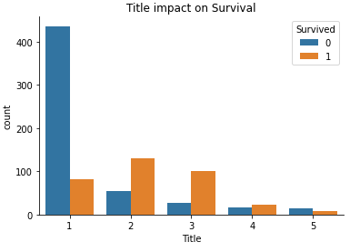
sns.countplot(x ='Title', hue = "Survived", data = train_data).set_title("Title impact on Survival")
sns.despine()
number_column = ["Fare"]
# Imputing Fare
from sklearn.impute import SimpleImputer

# Imputation of number columns.
my_imputer = SimpleImputer()

train_data[number_column] = pd.DataFrame(my_imputer.fit_transform(train_data[number_column]))

test_data[number_column] = pd.DataFrame(my_imputer.transform(test_data[number_column]))
train_data['FareBand'] = pd.qcut(train_data['Fare'], 4)
test_data['FareBand'] = pd.qcut(test_data['Fare'], 4)

#creating FareBand column
def fare_fun(row):
    if row <= 7.91:
        return 0
    elif row > 7.91 and row <= 14.454:
        return 1
    elif row > 14.454 and row <= 31:
        return 2
    else:
        return 3

train_data["FareBand"] = train_data["Fare"].apply(fare_fun)
test_data["FareBand"] = test_data["Fare"].apply(fare_fun)
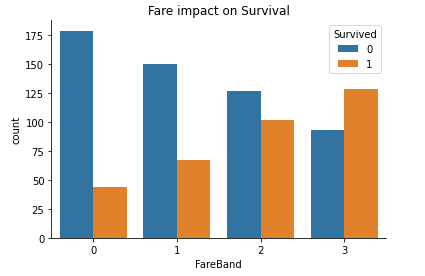
sns.countplot(x ='FareBand', hue = "Survived", data = train_data).set_title("Fare impact on Survival")
sns.despine()
Looking at all the above plots we can now deduce on what variable that we can use to predict survival based on their impact on the same. We see that “Pclass”, “Sex”, “SibSp”, “Parch”, “Title”, “Fare” have quite a significant influence on the target variate hence we can proceed to make use of them in the model
Random Forest
This is a supervised kind of learning algorithm. It averages the result from different decision trees i.e an ensemble of decision trees. They combine multiple trees to predict the class of the dataset.
from sklearn.ensemble import RandomForestClassifier

y = train_data["Survived"]

features = ["Pclass", "Sex", "SibSp", "Parch", "Title", "Fare"]
X = pd.get_dummies(train_data[features])
X_test = pd.get_dummies(test_data[features])

model = RandomForestClassifier(n_estimators=100, max_depth=5, random_state=1)
model.fit(X, y)
predictions = model.predict(X_test)

output = pd.DataFrame({'PassengerId': test_data.PassengerId, 'Survived': predictions})
output.to_csv('my_submission.csv', index=False)
