Value at Risk
Value at Risk (VaR) is a risk management tool used to estimate the potential loss of an investment portfolio over a specified time horizon given a certain confidence level (of the analyst, the most used being 95%). The basic idea behind VaR is to provide a single number that summarizes the potential downside risk of an investment portfolio. The VaR is calculated by modeling the distribution of returns for a portfolio and then determining the level of loss that is exceeded with a given degree of confidence.
For instance, if the Value at Risk of a portfolio is 1 million with a 95% confidence level, it implies that there is a 5% chance that the portfolio will lose more than 1 million over the specified time horizon. VaR is widely used in the finance industry to measure and manage market risk.
There are several methods to calculate VaR, including the Variance-Covariance Method, the Historical Simulation Method, and the Monte Carlo Simulation Method. The choice of the method to implement usually depends on the characteristics of the portfolio and the goals of the risk management exercise.
Methodologies
Historical simulation:This method uses historical data to simulate future returns and calculates the VaR based on the worst losses over the specified time horizon and confidence level.Variance-covariance method:This method assumes a normal distribution of returns and calculates VaR based on the portfolio’s mean and standard deviation.Monte Carlo simulation:This method uses statistical simulations to generate random future returns based on historical data and calculates the VaR based on the worst losses over the specified time horizon and confidence level.Extreme value theory:This method assumes that the distribution of returns is not normal and uses statistical models to estimate the likelihood of extreme losses.Parametric methods:These methods assume a specific distribution of returns and use that distribution to estimate VaR. For example, the variance-covariance method assumes a normal distribution, while the historical simulation method does not make any assumptions about the distribution of returns.Modified VaR (CVaR):This method is a variation of VaR that takes into account the expected loss in addition to the potential loss. CVaR provides a more comprehensive estimate of portfolio risk than VaR alone.Filtered Historical Simulation (FHS):This method combines the benefits of historical simulation and Monte Carlo simulation, by using a historical dataset to estimate the distribution of returns and then generating simulations based on that distribution.Exponentially Weighted Moving Average (EWMA):This method uses a weighted average of past returns to estimate the mean and volatility of returns, which are then used to calculate VaR.Implied Volatility Method:This method uses option prices to estimate the implied volatility of the underlying assets and then uses that information to calculate VaR.Kernel Density Estimation (KDE):This method uses a non-parametric approach to estimate the distribution of returns and calculate VaR based on that distribution.Backtesting:This method uses historical data to validate the accuracy of VaR calculations by comparing the estimated VaR with actual losses.Incremental VaR (IVaR):This method calculates VaR incrementally, by considering the impact of each trade on the portfolio’s VaR.Hybrid methods:These methods combine two or more of the above methodologies to estimate VaR.
Few Instances in Python
Quantile based VAR
A quantile-based histogram plot with returns and Value-at-Risk (VaR) is a visualization tool that helps to assess the risk associated with a portfolio of financial assets.
# Dependencies
import numpy as np
import pandas as pd
import matplotlib.pyplot as plt


import arch.data.sp500
from arch import arch_model
plt.style.use('ggplot')


# data
data = arch.data.sp500.load()
market = data["Adj Close"]
returns = 100 * market.pct_change().dropna()


# Define the confidence level
confidence_level = 0.05

# Calculate VaR using the quantile method
var = -np.percentile(returns, 100 * confidence_level)
print('Value at Risk:', var)

# Plot the returns distribution
plt.hist(returns, bins=50, density=True, label='Returns')
plt.axvline(x=var, color='red', label='VaR')
plt.legend()
plt.show()
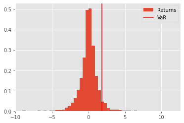
This code first loads stock price data from arch package to a Pandas DataFrame. The returns for the stock are calculated as the percentage change in the adjusted close price. The np.percentile function is used to calculate the VaR for a specified confidence level (in this case, 95%). The VaR is calculated as the quantile that corresponds to the specified confidence level. Finally, a histogram of the returns is plotted, and the VaR is indicated with a red vertical line.
The code above yields a VAR of 1.8643329744495285, which represents the threshold value below which the portfolio is expected to incur losses with a confidence of 95%.
The yielded plot:

The X-axis represents the quantiles or percentiles of the returns distribution, while the Y-axis represents the magnitude of returns. The plot shows the frequency or density of returns at different levels of quantiles, which gives one an idea of how the returns are distributed across different levels of risk.
The Value-at-Risk (VaR) line is plotted on the histogram to represent the level of risk associated with a confidence level of 95% (one can have another confidence despite the 95%). The VaR line represents the threshold beyond which the portfolio is expected to incur losses with 95% confidence.
Parametric VAR
A parametric Value at Risk (VaR) plot is a graphical representation of the VaR of a portfolio over a specified time horizon and confidence level.
Python Code
# Dependencies
import arch.data.sp500
from arch import arch_model
import pandas as pd
import numpy as np
import matplotlib.pyplot as plt
plt.style.use('ggplot')


# data
data = arch.data.sp500.load()
market = data["Adj Close"]
returns = 100 * market.pct_change().dropna()

# defining model
am = arch_model(returns, vol="Garch", p=1, o=0, q=1, dist="skewt")
res = am.fit(disp="off", last_obs="2017-12-31")

# forecasting
forecasts = res.forecast(start="2018-1-1", reindex=False)
cond_mean = forecasts.mean["2018":]
cond_var = forecasts.variance["2018":]
q = am.distribution.ppf([0.01, 0.05], res.params[-2:])
print(q)

# VAR
value_at_risk = -cond_mean.values - np.sqrt(cond_var).values * q[None, :]
value_at_risk = pd.DataFrame(value_at_risk, columns=["1%", "5%"], index=cond_var.index)
ax = value_at_risk.plot(legend=False)
xl = ax.set_xlim(value_at_risk.index[0], value_at_risk.index[-1])
rets_2018 = returns["2018":].copy()
rets_2018.name = "S&P 500 Return"
c = []
for idx in value_at_risk.index:
    if rets_2018[idx] > -value_at_risk.loc[idx, "5%"]:
        c.append("#000000")
    elif rets_2018[idx] < -value_at_risk.loc[idx, "1%"]:
        c.append("#BB0000")
    else:
        c.append("#BB00BB")
c = np.array(c, dtype="object")
labels = {"#BB0000": "1% Exceedence", "#BB00BB": "5% Exceedence", "#000000": "No Exceedence",}
markers = {"#BB0000": "x", "#BB00BB": "s", "#000000": "o"}
for color in np.unique(c):
    sel = c == color
    ax.scatter(
        rets_2018.index[sel],
        -rets_2018.loc[sel],
        marker=markers[color],
        c=c[sel],
        label=labels[color],
    )
ax.set_title("Parametric VaR")
leg = ax.legend(frameon=False, ncol=3)
plt.show()
Which yields the plot:

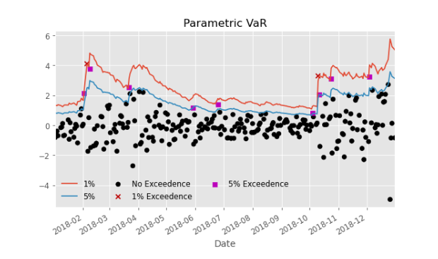
The plot helps to assess the level of risk associated with the portfolio at different points in time and to understand how the risk evolves over time.
The X-axis representing time, and the Y-axis representing the estimated VaR value for each time point. The plot shows how the VaR evolves over time and helps to identify any trends or patterns in the risk profile of the portfolio.
The interpretation of the plot can be as follows:
- The slope of the VaR line indicates the rate of change in the level of risk over time. A rising slope indicates that the risk is increasing over time, while a declining slope indicates that the risk is decreasing over time.
- The level of the VaR line represents the overall level of risk associated with the portfolio. A higher VaR value indicates a higher level of risk, while a lower VaR value indicates a lower level of risk.
- The plot can help to identify any spikes or spikes in the VaR values as in the figure above, which may indicate events or conditions that are affecting the risk profile of the portfolio.
Summary
Value-at-Risk (VaR) is a widely used risk management metric that provides a statistical estimate of the potential loss of a portfolio over a specified time horizon and confidence level. VaR represents the maximum loss that can be expected with a specified level of confidence.
VaR is used by investors and risk managers to assess the level of risk associated with a portfolio and to make informed investment decisions. A lower VaR value indicates a lower level of risk, while a higher VaR value indicates a higher level of risk. VaR is a useful tool for managing and reducing risk in a portfolio, and for understanding the potential impact of market changes on a portfolio’s performance.
VaR calculations can be based on various statistical methods, including historical simulation, Monte Carlo simulation, and parametric methods.